Offline analysis

Ask questions of a recorded session: where did the robot go, what did it see, and where is the thing I care about

After a run you have a recording - a memory2 .db from Record & replay holding every camera frame, lidar scan, and pose from the session. This page is about asking that file questions:

• Where did the robot go, and how fast? Debug navigation without re-running the robot.
• What did the environment look like? Map room lighting, coverage, sensor quality.
• When and where did the robot see X? Search hours of video with a sentence, then jump straight to those frames and places.

That last one is the headline capability: recorded vision becomes a searchable index. Instead of scrubbing video, you type “plant” and get back timestamps, map locations, and the frames themselves.

Everything below is an executable notebook (the code blocks run for real in CI) working on go2_bigoffice, a bundled five-minute Go2 drive around an office. Swap in your own recording and everything works the same. The query API used throughout is documented in The memory2 library.

The session

Open the store and see what was recorded:

Python

store = SqliteStore(path=get_data("go2_bigoffice.db"))

for name, stream in store.streams.items():
   print(stream.summary())

Stream("color_image"): 4164 items, 2025-12-26 11:09:08 - 2025-12-26 11:14:00 (292.5s)
Stream("color_image_embedded"): 267 items, 2025-12-26 11:09:12 - 2025-12-26 11:14:00 (288.4s)
Stream("lidar"): 2251 items, 2025-12-26 11:09:08 - 2025-12-26 11:14:00 (292.3s)
Stream("odom"): 5465 items, 2025-12-26 11:09:08 - 2025-12-26 11:14:00 (292.5s)

Five minutes of driving: 4k camera frames, 2k lidar scans, 5k odometry samples. Every observation carries its timestamp and the robot’s pose, which is what makes the spatial queries below possible.

Draw where the robot went

Space is a top-down spatial canvas: add any stream to it and each observation is drawn at the pose where it was captured, colored by time (turbo colormap, blue early to red late). Adding the camera stream literally draws the robot’s trajectory:

Python

global_map = pickle.loads(get_data("unitree_go2_bigoffice_map.pickle").read_bytes())

drawing = Space()

# this is not necessary but we use a global map as a nice base for a drawing
drawing.add(global_map)
drawing.add(store.streams.color_image)
drawing.to_svg("assets/color_image.svg")

One glance answers: what was covered, where the robot lingered, whether it doubled back.

Derive new streams

Queries are lazy stream pipelines: .transform() and .map() build new streams from recorded ones without touching the database until you draw or iterate. Two practical examples.

How fast was the robot moving, where? Useful for spotting where navigation slowed down or got stuck:

Python

drawing = Space()
drawing.add(global_map)

drawing.add(
  store.streams.color_image \
  # calculate speed in m/s by checking distance between poses and timestamps of observations
  .transform(speed()) \
  # rolling window average
  .transform(smooth(50)))

drawing.to_svg("assets/speed.svg")

What is the lighting like around the space? Any per-frame quantity can be painted onto the map the same way - here, image brightness. This kind of environment map matters later: dark frames are useless for vision, and we will filter on exactly this signal before embedding:

Python

drawing = Space()
drawing.add(global_map)

drawing.add(
  store.streams.color_image \
  # here we will take 4fps because brightness calculation loads the actual image
  # observation.data triggers another db query to fetch the data
  # otherwise observations only hold positions and timestamps
  .transform(throttle(0.25)) \
  # we calculate brightness
  .map(lambda obs: obs.derive(data=obs.data.brightness)))

drawing.to_svg("assets/brightness.svg")

Make the camera stream searchable

To search video with text, embed the frames with CLIP once and save the result as a new stream in the same store. The pipeline filters dark frames (see the lighting map above), picks the sharpest frame in each half-second window, embeds, and saves:

Python

from dimos.models.embedding.clip import CLIPModel
from dimos.msgs.sensor_msgs.Image import Image
from dimos.memory2.transform import QualityWindow
from dimos.memory2.embed import EmbedImages

embedded = store.stream("color_image_embedded", Image)
clip = CLIPModel()

# Downsample to 2Hz, filter dark images, then embed
pipeline = (
    store.streams.color_image.filter(lambda obs: obs.data.brightness > 0.1)
    .transform(QualityWindow(lambda img: img.sharpness, window=0.5))
    .transform(EmbedImages(clip))
    .save(embedded)
)

print(pipeline)

Pipelines are lazy - execute by iterating, or with .drain():

skip

for obs in pipeline:
    print(f"  [{count}] ts={obs.ts:.2f} pose={obs.pose}")

Our bundled dataset already contains this color_image_embedded stream (267 embedded frames of the 4164 recorded).

Search by text

Now the session is queryable in natural language. Embed a text query and search - matches come back as ordinary observations, so they draw on the map like anything else:

Python

from dimos.models.embedding.clip import CLIPModel

drawing = Space()
drawing.add(global_map)

clip = CLIPModel()
search_vector = clip.embed_text("shop")
drawing.add(store.streams.color_image_embedded.search(search_vector))

drawing.to_svg("assets/embedding.svg")

We can go further: take the top matches, pull only the lidar captured at those moments, and reconstruct just the geometry around them - a focused 3D view of “the places that look like a shop”:

Python

from dimos.models.embedding.clip import CLIPModel
from dimos.mapping.voxels import VoxelMapTransformer
drawing = Space()

# this is defined here, but not executed
matches = store.streams.color_image_embedded.search(search_vector, k=30)

print(matches) # Stream("color_image_embedded") | vector_search(k=50)

# here we execute it once, and feed it into a global mapper, then draw the map
drawing.add(
   matches.map(lambda obs: store.streams.lidar.at(obs.ts).last()) \
   .transform(VoxelMapTransformer()) \
   .last().data)

# then we add matches to the map
drawing.add(matches)

drawing.to_svg("assets/embedding_focused.svg")

Stream("color_image_embedded") | vector_search(k=30)
13:15:15.190 [inf][dimos/mapping/voxels.py       ] VoxelGrid using device: CUDA:0

And view the matching frames themselves:

Python

plot_mosaic(matches.map(lambda obs: obs.data).to_list(), "assets/grid.png")

Search, locate, look - the whole point of pose-stamped recording in three cells.

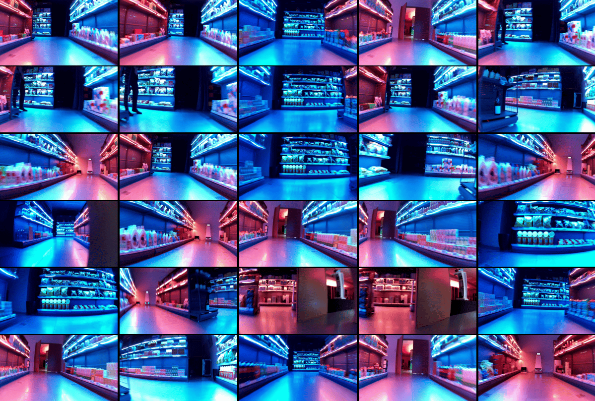
Case study: find the plants

A full worked example, end to end: did the robot see plants during the session, where exactly are they in the building, and can we verify with a detector? This is the workflow for any “find X in my recordings” task. It also plots over time rather than space, using the Plot API (time-series companion to Space).

First, a feel for the session on a timeline - speed, brightness, and elapsed time on separate axes:

session=robotdata output=none

from dimos.memory2.store.sqlite import SqliteStore
from dimos.memory2.transform import smooth, speed, throttle
from dimos.memory2.vis import color
from dimos.memory2.vis.plot.elements import Series
from dimos.memory2.vis.plot.plot import Plot
from dimos.utils.data import get_data

store = SqliteStore(path=get_data("go2_bigoffice.db"))
images = store.streams.color_image

plot = Plot()
plot.add(
    images.transform(speed()).transform(smooth(40)),
    label="speed (m/s)",
    opacity=0.75
)

plot.add(
    images.transform(throttle(0.5)).map_data(lambda obs: obs.data.brightness).transform(smooth(10)),
    label="brightness",
    color=color.blue,
)

plot.add(
    images.transform(throttle(0.5)).scan_data(images.first().ts, lambda state, obs: [state, obs.ts - state]),
    label="time",
    axis="time",
    opacity=0.5
)

plot.to_svg("assets/plot_robot_data.svg")

Score every frame against “plant”

Search the embedded stream and re-sort by time, giving a “plant-ness over the session” signal:

session=robotdata

from dimos.memory2.vis.plot.elements import Series, HLine, Style
from dimos.memory2.vis import color
from dimos.memory2.transform import normalize, smooth_time

from dimos.models.embedding.clip import CLIPModel
clip = CLIPModel()
search_vector = clip.embed_text("plant")

# we will cache this into memory since it takes a second,
# and use it to play with graphing
plantness_query = (
    store.streams.color_image_embedded
        .search(search_vector)
        # search() returns observations sorted by similarity, we re-sort by time
        .order_by("ts")
)

# we've built our query
print(plantness_query)

# we evaluate it into a in-memory stream,
# since we want to further process/plot multiple times
plantness_query_materialized = plantness_query.materialize()

print(plantness_query_materialized)
print(plantness_query_materialized.summary())

# let's create a numerical stream
plantness_similarity = plantness_query_materialized.map_data(lambda obs: obs.similarity).materialize()

plot = Plot()

plot.add(plantness_similarity,
  label="plant-ness",
  color=color.green,
)

plot.to_svg("assets/plot_plantness.svg")

Stream("color_image_embedded") | vector_search() | order_by(ts)
Stream("materialize")
Stream("materialize"): 267 items, 2025-12-26 11:09:12 - 2025-12-26 11:14:00 (288.4s)

There are clear peaks at the beginning and end of the run - but the graph is gappy and ugly. Why?

Embeddings were only computed above a minimum brightness. Completely dark images are both useless and semantically close to everything. Overlay brightness to confirm the gaps line up:

session=robotdata

plot = Plot()

plot.add(plantness_similarity,
  label="plant-ness",
  color=color.green,
)

plot.add(
    images.transform(throttle(0.5)).map_data(lambda obs: obs.data.brightness),
    label="brightness",
    axis="brightness"
)

plot.add(HLine(y=0.15, style=Style.dashed, color=color.red))

plot.to_svg("assets/plot_plantness_brightness.svg")

Nothing is embedded below the brightness floor. Clean the signal up: treat unmapped values as zero, connect points within 7.5 s, smooth over a 5 s window, normalize:

session=robotdata

plot = Plot()

plot.add(
    plantness_similarity \
      .transform(smooth_time(5.0)) \
      .transform(normalize()), \
      label="plant-ness",
      color=color.green,
      gap_fill=0.0,
      connect=7.5
)

plot.to_svg("assets/plot_plantness_gap_fill.svg")

Auto-detect the peaks and verify with a VLM

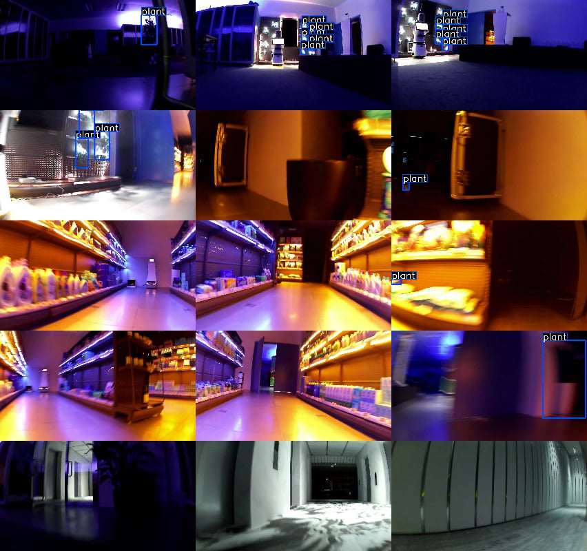
Obvious peaks. Auto-detect them, pull the frames at those moments, and run a detector (Moondream, one of the VLM backends) to verify there really are plants:

skip session=robotdata

from dimos.mapping.voxels import VoxelMapTransformer
from dimos.memory2.vis.space.space import Space
from dimos.memory2.transform import peaks
from dimos.memory2.vis.color import ColorRange
from dimos.memory2.vis.plot.elements import VLine
from dimos.memory2.vis.utils import mosaic
from dimos.memory2.stream import Stream
from itertools import chain

semantic_peaks = plantness_query_materialized.transform(peaks(key=lambda obs: obs.similarity, distance=1.0))

# load all lidar frames captured in the readius around the semantic peaks
# feed them into a global mapper to get a single pointcloud around our areas of interest
global_map = semantic_peaks \
   .map(lambda obs: store.streams.lidar.near(obs.pose_stamped, radius=0.5).first()) \
   .transform(VoxelMapTransformer()) \
   .last().data

drawing = Space()
drawing.add(global_map)
drawing.add(semantic_peaks)
drawing.to_svg("assets/plot_plantness_autopeaks_map.svg")

peakColor = ColorRange("turbo")
for i, p in enumerate(semantic_peaks):
    print(f"t={p.ts - plantness_similarity.first().ts:6.1f}s score={p.similarity:.3f} prominence={p.tags['peak_prominence']:.3f}")
    plot.add(VLine(p.ts, color=peakColor(i)))

plot.to_svg("assets/plot_plantness_autopeaks.svg")

from dimos.models.vl.moondream import MoondreamVlModel
moondream = MoondreamVlModel()
moondream.start()

# peaks is still a stream of image observations (with prominence and semantic similarity metadata)
# so we can just draw it directly via mosaic that takes image streams
m = mosaic(semantic_peaks.map_data(lambda obs: moondream.query_detections(obs.data, "plant")))

m.data.save("assets/plants_auto.png")

14:59:33.042 [inf][dimos/mapping/voxels.py       ] VoxelGrid using device: CUDA:0
t=  14.1s score=0.224 prominence=0.031
t=  26.3s score=0.225 prominence=0.033
t=  32.7s score=0.224 prominence=0.022
t=  37.0s score=0.259 prominence=0.067
t=  60.6s score=0.227 prominence=0.031
t=  61.5s score=0.218 prominence=0.026
t=  76.3s score=0.221 prominence=0.031
t=  84.0s score=0.223 prominence=0.027
t=  89.1s score=0.219 prominence=0.020
t= 162.9s score=0.224 prominence=0.041
t= 168.0s score=0.219 prominence=0.031
t= 172.4s score=0.218 prominence=0.020
t= 240.4s score=0.243 prominence=0.047
t= 245.6s score=0.224 prominence=0.028
t= 279.6s score=0.230 prominence=0.030

Which peaks are significant?

We got 15 peaks back. Most prominences sit around 0.02-0.03 and only a couple (0.067 at t=37s, 0.047 at t=240s) really stand out. significant() replaces eyeballing that cutoff by thresholding on the distribution of prominences itself (default: MAD, median absolute deviation).

Once the surviving peaks go on the timeline, we get two very obvious plants:

skip session=robotdata

from dimos.memory2.transform import significant

plot = Plot()
plot.add(
    plantness_similarity.transform(smooth_time(5.0)).transform(normalize()),
    label="plant-ness", color=color.green, gap_fill=0.0, connect=7.5,
)

meaningful_peaks = semantic_peaks.transform(significant(method="mad"))

for peak in meaningful_peaks:
    plot.add(VLine(peak.ts, color=color.red))

m = mosaic(meaningful_peaks)
m.data.save("assets/plants_meaningful.png")

plot.to_svg("assets/plot_plantness_significant.svg")

Rule of thumb: keep a small absolute floor on peaks(prominence=...) to reject shape-noise, then let significant() pick the statistical cutoff.

Zoom into a hotspot

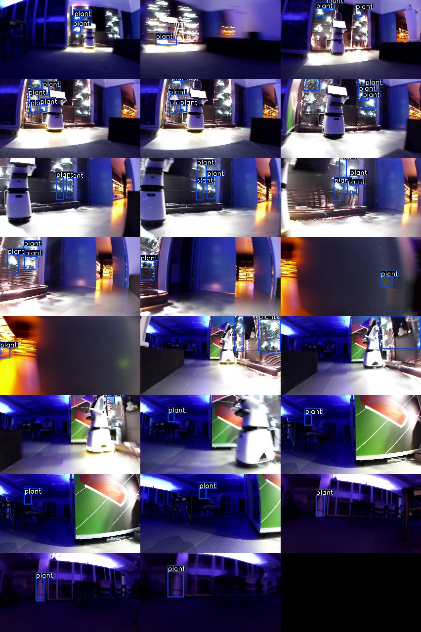
Focus on the strongest peak: load every image captured within 2.5 m of it (filtered for brightness and sharpness), rebuild the local 3D map from the lidar around it, and run the detector on all nearby views:

skip session=robotdata

from dimos.memory2.vis.space.elements import Point
from dimos.memory2.transform import QualityWindow

drawing = Space()

# TODO actual near/at filters need to accept observation streams in order to easily
# reconstruct all frames in vicinity of another stream
# for now for simplicity here we are focusing only on one semantic hotspot.
meaningful_peak = meaningful_peaks.first()

# load all images captured in the readius around the semantic peak
near_images = images.near(meaningful_peak.pose_stamped, radius=2.5) \
    .filter(lambda obs: obs.data.brightness > 0.1) \
    .transform(QualityWindow(lambda img: img.sharpness, window=0.5))

# load all lidar frames captured in the readius around the semantic peak
# feed them into a global mapper to get a single pointcloud around our area of interest
global_map = store.streams.lidar.near(meaningful_peak.pose_stamped, radius=2.5) \
   .transform(VoxelMapTransformer()) \
   .last().data

# run our global mapper only on lidar frames around the POI
drawing.add(global_map)
drawing.add(meaningful_peak.pose_stamped, color=color.green)

# run a detector, filter small weird detections
detections = (near_images
    .map_data(lambda obs: moondream.query_detections(obs.data, "plant"))
    .map_data(lambda obs: obs.data.filter(lambda det: det.bbox_2d_volume() > 3000))
    .filter(lambda obs: len(obs.data) > 0)
    .materialize())
    # materialize this stream since we'll want to re-use it later

drawing.add(detections)
drawing.to_svg("assets/peak_space.svg")

m = mosaic(detections)
m.data.save("assets/plants_peak_detections.png")

Project detections into 3D

Finally, lift the 2D detections into 3D boxes on the map using the camera model and the pointcloud - from “the robot saw a plant at t=37s” to “there is a plant here”:

skip session=robotdata output=none

from dimos.perception.detection.type.detection3d.imageDetections3DPC import (
    ImageDetections3DPC,
)
from dimos.robot.unitree.go2.connection import (
    _camera_info_static as go2_camerainfo,
    BASE_TO_OPTICAL,
)
from dimos.memory2.vis.space.elements import Box3D
from dimos.msgs.geometry_msgs.Pose import Pose
from dimos.msgs.geometry_msgs.Transform import Transform
from dimos.msgs.geometry_msgs.Vector3 import Vector3

# TODO We need a nicer way to get optical transform for image streams
# depending on the source
def world_to_optical(base_pose):
    return -(Transform.from_pose("base_link", base_pose) + BASE_TO_OPTICAL)

drawing = Space()

drawing.add(global_map)

drawing.add(detections)

camera_info = go2_camerainfo()

detections3d = (detections
    .map_data(lambda obs: ImageDetections3DPC.from_2d(
        obs.data,
        global_map,
        camera_info,
        world_to_optical(obs.pose_stamped),
    ))
    .filter(lambda obs: len(obs.data) > 0))

# TODO detection3d needs to be a natural thing to render
for obs in detections3d:
    for d3d in obs.data:
        aabb = d3d.get_bounding_box()
        c, e = aabb.get_center(), aabb.get_extent()
        drawing.add(Box3D(
            center=Pose(float(c[0]), float(c[1]), float(c[2])),
            size=Vector3(float(e[0]), float(e[1]), float(e[2])),
            color=color.green, label="plant",
        ))

drawing.to_svg("assets/peak_detections.svg")

That is the full loop: text query, temporal peaks, spatial hotspot, verified detections, 3D locations - all from one recorded drive, none of it requiring the robot again.

Appendix: plotting API notes

Small things worth knowing about Plot when you build your own analyses.

Colors auto-cycle as you add series:

session=plot output=none

import math
import random

from dimos.memory2.vis.plot.elements import Series
from dimos.memory2.vis.plot.plot import Plot

rng = random.Random(42)
xs = [i * 0.1 for i in range(120)]

color_check = Plot()
for i in range(14):
    phase = rng.uniform(0, 2 * math.pi)
    freq = rng.uniform(0.5, 1.8)
    amp = rng.uniform(0.6, 1.4)
    offset = i * 0.5  # vertical separation so curves don't overlap
    ys = [amp * math.sin(freq * x + phase) + offset for x in xs]

    color_check.add(Series(ts=xs, values=ys, label=f"curve {i + 1}"))

color_check.to_svg("assets/plot_colors.svg")

Named colors can also be used explicitly. When you pin a series to one of the named colors, the auto-cycle excludes it for the remaining series, so you never end up with two lines that share a color by accident:

session=plot output=none

from dimos.memory2.vis import color
from dimos.memory2.vis.plot.elements import Series, HLine, Style

p = Plot()
# auto -> blue
p.add(Series(ts=xs, values=[math.sin(x) for x in xs]))
# explicit green, dotted
p.add(Series(ts=xs, values=[math.cos(x) for x in xs], color=color.red, style=Style.dotted))
# auto -> yellow (red is excluded)
p.add(Series(ts=xs, values=[math.sin(2 * x) for x in xs]))
# explicit color
p.add(HLine(y=0, style=Style.dashed, opacity=0.5, color="#ff0000"))
p.to_svg("assets/plot_named.svg")