> ## Documentation Index
> Fetch the complete documentation index at: https://dimensionalos.mintlify.site/llms.txt
> Use this file to discover all available pages before exploring further.
# Offline analysis
> Ask questions of a recorded session: where did the robot go, what did it see, and where is the thing I care about
After a run you have a recording - a memory2 `.db` from [Record & replay](/capabilities/memory/record-and-replay) holding every camera frame, lidar scan, and pose from the session. This page is about asking that file questions:
* **Where did the robot go, and how fast?** Debug navigation without re-running the robot.
* **What did the environment look like?** Map room lighting, coverage, sensor quality.
* **When and where did the robot see X?** Search hours of video with a sentence, then jump straight to those frames and places.
That last one is the headline capability: recorded vision becomes a searchable index. Instead of scrubbing video, you type "plant" and get back timestamps, map locations, and the frames themselves.
Everything below is an executable notebook (the code blocks run for real in CI) working on `go2_bigoffice`, a bundled five-minute Go2 drive around an office. Swap in your own recording and everything works the same. The query API used throughout is documented in [The memory2 library](/capabilities/memory/memory2-library).
## The session
Open the store and see what was recorded:
Python
```python title="Python" fold session=mem output=none theme={null}
import pickle
from dimos.mapping.pointclouds.occupancy import general_occupancy, simple_occupancy, height_cost_occupancy
from dimos.mapping.occupancy.inflation import simple_inflate
from dimos.memory2.store.sqlite import SqliteStore
from dimos.memory2.vis.color import Color
from dimos.memory2.transform import downsample, throttle, speed, smooth
from dimos.memory2.vis.space.space import Space
from dimos.utils.data import get_data
from dimos.memory2.vis.space.elements import Point
```
```python title="Python" session=mem theme={null}
store = SqliteStore(path=get_data("go2_bigoffice.db"))
for name, stream in store.streams.items():
print(stream.summary())
```
```results theme={null}
Stream("color_image"): 4164 items, 2025-12-26 11:09:08 - 2025-12-26 11:14:00 (292.5s)
Stream("color_image_embedded"): 267 items, 2025-12-26 11:09:12 - 2025-12-26 11:14:00 (288.4s)
Stream("lidar"): 2251 items, 2025-12-26 11:09:08 - 2025-12-26 11:14:00 (292.3s)
Stream("odom"): 5465 items, 2025-12-26 11:09:08 - 2025-12-26 11:14:00 (292.5s)
```
Five minutes of driving: 4k camera frames, 2k lidar scans, 5k odometry samples. Every observation carries its timestamp and the robot's pose, which is what makes the spatial queries below possible.
## Draw where the robot went
`Space` is a top-down spatial canvas: add any stream to it and each observation is drawn at the pose where it was captured, colored by time (turbo colormap, blue early to red late). Adding the camera stream literally draws the robot's trajectory:
```python title="Python" session=mem output=none theme={null}
global_map = pickle.loads(get_data("unitree_go2_bigoffice_map.pickle").read_bytes())
drawing = Space()
# this is not necessary but we use a global map as a nice base for a drawing
drawing.add(global_map)
drawing.add(store.streams.color_image)
drawing.to_svg("assets/color_image.svg")
```
 One glance answers: what was covered, where the robot lingered, whether it doubled back.
## Derive new streams
Queries are lazy stream pipelines: `.transform()` and `.map()` build new streams from recorded ones without touching the database until you draw or iterate. Two practical examples.
**How fast was the robot moving, where?** Useful for spotting where navigation slowed down or got stuck:
```python title="Python" session=mem output=none theme={null}
drawing = Space()
drawing.add(global_map)
drawing.add(
store.streams.color_image \
# calculate speed in m/s by checking distance between poses and timestamps of observations
.transform(speed()) \
# rolling window average
.transform(smooth(50)))
drawing.to_svg("assets/speed.svg")
```
One glance answers: what was covered, where the robot lingered, whether it doubled back.
## Derive new streams
Queries are lazy stream pipelines: `.transform()` and `.map()` build new streams from recorded ones without touching the database until you draw or iterate. Two practical examples.
**How fast was the robot moving, where?** Useful for spotting where navigation slowed down or got stuck:
```python title="Python" session=mem output=none theme={null}
drawing = Space()
drawing.add(global_map)
drawing.add(
store.streams.color_image \
# calculate speed in m/s by checking distance between poses and timestamps of observations
.transform(speed()) \
# rolling window average
.transform(smooth(50)))
drawing.to_svg("assets/speed.svg")
```
 **What is the lighting like around the space?** Any per-frame quantity can be painted onto the map the same way - here, image brightness. This kind of environment map matters later: dark frames are useless for vision, and we will filter on exactly this signal before embedding:
```python title="Python" session=mem output=none theme={null}
drawing = Space()
drawing.add(global_map)
drawing.add(
store.streams.color_image \
# here we will take 4fps because brightness calculation loads the actual image
# observation.data triggers another db query to fetch the data
# otherwise observations only hold positions and timestamps
.transform(throttle(0.25)) \
# we calculate brightness
.map(lambda obs: obs.derive(data=obs.data.brightness)))
drawing.to_svg("assets/brightness.svg")
```
**What is the lighting like around the space?** Any per-frame quantity can be painted onto the map the same way - here, image brightness. This kind of environment map matters later: dark frames are useless for vision, and we will filter on exactly this signal before embedding:
```python title="Python" session=mem output=none theme={null}
drawing = Space()
drawing.add(global_map)
drawing.add(
store.streams.color_image \
# here we will take 4fps because brightness calculation loads the actual image
# observation.data triggers another db query to fetch the data
# otherwise observations only hold positions and timestamps
.transform(throttle(0.25)) \
# we calculate brightness
.map(lambda obs: obs.derive(data=obs.data.brightness)))
drawing.to_svg("assets/brightness.svg")
```
 ## Make the camera stream searchable
To search video with text, embed the frames with CLIP once and save the result as a new stream in the same store. The pipeline filters dark frames (see the lighting map above), picks the sharpest frame in each half-second window, embeds, and saves:
```python title="Python" session=mem skip theme={null}
from dimos.models.embedding.clip import CLIPModel
from dimos.msgs.sensor_msgs.Image import Image
from dimos.memory2.transform import QualityWindow
from dimos.memory2.embed import EmbedImages
embedded = store.stream("color_image_embedded", Image)
clip = CLIPModel()
# Downsample to 2Hz, filter dark images, then embed
pipeline = (
store.streams.color_image.filter(lambda obs: obs.data.brightness > 0.1)
.transform(QualityWindow(lambda img: img.sharpness, window=0.5))
.transform(EmbedImages(clip))
.save(embedded)
)
print(pipeline)
```
Pipelines are lazy - execute by iterating, or with `.drain()`:
```python skip theme={null}
for obs in pipeline:
print(f" [{count}] ts={obs.ts:.2f} pose={obs.pose}")
```
Our bundled dataset already contains this `color_image_embedded` stream (267 embedded frames of the 4164 recorded).
## Search by text
Now the session is queryable in natural language. Embed a text query and search - matches come back as ordinary observations, so they draw on the map like anything else:
```python title="Python" session=mem output=none theme={null}
from dimos.models.embedding.clip import CLIPModel
drawing = Space()
drawing.add(global_map)
clip = CLIPModel()
search_vector = clip.embed_text("shop")
drawing.add(store.streams.color_image_embedded.search(search_vector))
drawing.to_svg("assets/embedding.svg")
```
## Make the camera stream searchable
To search video with text, embed the frames with CLIP once and save the result as a new stream in the same store. The pipeline filters dark frames (see the lighting map above), picks the sharpest frame in each half-second window, embeds, and saves:
```python title="Python" session=mem skip theme={null}
from dimos.models.embedding.clip import CLIPModel
from dimos.msgs.sensor_msgs.Image import Image
from dimos.memory2.transform import QualityWindow
from dimos.memory2.embed import EmbedImages
embedded = store.stream("color_image_embedded", Image)
clip = CLIPModel()
# Downsample to 2Hz, filter dark images, then embed
pipeline = (
store.streams.color_image.filter(lambda obs: obs.data.brightness > 0.1)
.transform(QualityWindow(lambda img: img.sharpness, window=0.5))
.transform(EmbedImages(clip))
.save(embedded)
)
print(pipeline)
```
Pipelines are lazy - execute by iterating, or with `.drain()`:
```python skip theme={null}
for obs in pipeline:
print(f" [{count}] ts={obs.ts:.2f} pose={obs.pose}")
```
Our bundled dataset already contains this `color_image_embedded` stream (267 embedded frames of the 4164 recorded).
## Search by text
Now the session is queryable in natural language. Embed a text query and search - matches come back as ordinary observations, so they draw on the map like anything else:
```python title="Python" session=mem output=none theme={null}
from dimos.models.embedding.clip import CLIPModel
drawing = Space()
drawing.add(global_map)
clip = CLIPModel()
search_vector = clip.embed_text("shop")
drawing.add(store.streams.color_image_embedded.search(search_vector))
drawing.to_svg("assets/embedding.svg")
```
 We can go further: take the top matches, pull only the lidar captured at those moments, and reconstruct just the geometry around them - a focused 3D view of "the places that look like a shop":
```python title="Python" session=mem output=none theme={null}
from dimos.models.embedding.clip import CLIPModel
from dimos.mapping.voxels import VoxelMapTransformer
drawing = Space()
# this is defined here, but not executed
matches = store.streams.color_image_embedded.search(search_vector, k=30)
print(matches) # Stream("color_image_embedded") | vector_search(k=50)
# here we execute it once, and feed it into a global mapper, then draw the map
drawing.add(
matches.map(lambda obs: store.streams.lidar.at(obs.ts).last()) \
.transform(VoxelMapTransformer()) \
.last().data)
# then we add matches to the map
drawing.add(matches)
drawing.to_svg("assets/embedding_focused.svg")
```
```results theme={null}
Stream("color_image_embedded") | vector_search(k=30)
13:15:15.190 [inf][dimos/mapping/voxels.py ] VoxelGrid using device: CUDA:0
```
We can go further: take the top matches, pull only the lidar captured at those moments, and reconstruct just the geometry around them - a focused 3D view of "the places that look like a shop":
```python title="Python" session=mem output=none theme={null}
from dimos.models.embedding.clip import CLIPModel
from dimos.mapping.voxels import VoxelMapTransformer
drawing = Space()
# this is defined here, but not executed
matches = store.streams.color_image_embedded.search(search_vector, k=30)
print(matches) # Stream("color_image_embedded") | vector_search(k=50)
# here we execute it once, and feed it into a global mapper, then draw the map
drawing.add(
matches.map(lambda obs: store.streams.lidar.at(obs.ts).last()) \
.transform(VoxelMapTransformer()) \
.last().data)
# then we add matches to the map
drawing.add(matches)
drawing.to_svg("assets/embedding_focused.svg")
```
```results theme={null}
Stream("color_image_embedded") | vector_search(k=30)
13:15:15.190 [inf][dimos/mapping/voxels.py ] VoxelGrid using device: CUDA:0
```
 And view the matching frames themselves:
Python
```python title="Python" fold session=mem theme={null}
import matplotlib
import matplotlib.pyplot as plt
import math
def plot_mosaic(frames, path, cols=5):
matplotlib.use("Agg")
rows = math.ceil(len(frames) / cols)
aspect = frames[0].width / frames[0].height
fig_w, fig_h = 12, 12 * rows / (cols * aspect)
fig, axes = plt.subplots(rows, cols, figsize=(fig_w, fig_h))
fig.patch.set_facecolor("black")
for i, ax in enumerate(axes.flat):
if i < len(frames):
ax.imshow(frames[i].data)
for spine in ax.spines.values():
spine.set_color("black")
spine.set_linewidth(0)
ax.set_xticks([])
ax.set_yticks([])
else:
ax.axis("off")
plt.subplots_adjust(wspace=0.02, hspace=0.02, left=0, right=1, top=1, bottom=0)
plt.savefig(path, facecolor="black", dpi=100, bbox_inches="tight", pad_inches=0)
plt.close()
```
```python title="Python" session=mem theme={null}
plot_mosaic(matches.map(lambda obs: obs.data).to_list(), "assets/grid.png")
```
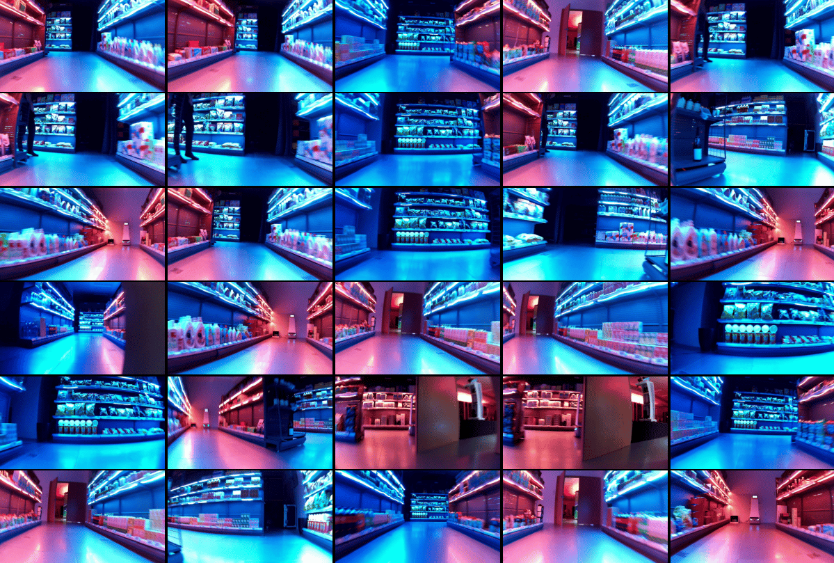 Search, locate, look - the whole point of pose-stamped recording in three cells.
## Case study: find the plants
A full worked example, end to end: did the robot see plants during the session, where exactly are they in the building, and can we verify with a detector? This is the workflow for any "find X in my recordings" task. It also plots over time rather than space, using the `Plot` API (time-series companion to `Space`).
First, a feel for the session on a timeline - speed, brightness, and elapsed time on separate axes:
```python session=robotdata output=none theme={null}
from dimos.memory2.store.sqlite import SqliteStore
from dimos.memory2.transform import smooth, speed, throttle
from dimos.memory2.vis import color
from dimos.memory2.vis.plot.elements import Series
from dimos.memory2.vis.plot.plot import Plot
from dimos.utils.data import get_data
store = SqliteStore(path=get_data("go2_bigoffice.db"))
images = store.streams.color_image
plot = Plot()
plot.add(
images.transform(speed()).transform(smooth(40)),
label="speed (m/s)",
opacity=0.75
)
plot.add(
images.transform(throttle(0.5)).map_data(lambda obs: obs.data.brightness).transform(smooth(10)),
label="brightness",
color=color.blue,
)
plot.add(
images.transform(throttle(0.5)).scan_data(images.first().ts, lambda state, obs: [state, obs.ts - state]),
label="time",
axis="time",
opacity=0.5
)
plot.to_svg("assets/plot_robot_data.svg")
```
Search, locate, look - the whole point of pose-stamped recording in three cells.
## Case study: find the plants
A full worked example, end to end: did the robot see plants during the session, where exactly are they in the building, and can we verify with a detector? This is the workflow for any "find X in my recordings" task. It also plots over time rather than space, using the `Plot` API (time-series companion to `Space`).
First, a feel for the session on a timeline - speed, brightness, and elapsed time on separate axes:
```python session=robotdata output=none theme={null}
from dimos.memory2.store.sqlite import SqliteStore
from dimos.memory2.transform import smooth, speed, throttle
from dimos.memory2.vis import color
from dimos.memory2.vis.plot.elements import Series
from dimos.memory2.vis.plot.plot import Plot
from dimos.utils.data import get_data
store = SqliteStore(path=get_data("go2_bigoffice.db"))
images = store.streams.color_image
plot = Plot()
plot.add(
images.transform(speed()).transform(smooth(40)),
label="speed (m/s)",
opacity=0.75
)
plot.add(
images.transform(throttle(0.5)).map_data(lambda obs: obs.data.brightness).transform(smooth(10)),
label="brightness",
color=color.blue,
)
plot.add(
images.transform(throttle(0.5)).scan_data(images.first().ts, lambda state, obs: [state, obs.ts - state]),
label="time",
axis="time",
opacity=0.5
)
plot.to_svg("assets/plot_robot_data.svg")
```
 ### Score every frame against "plant"
Search the embedded stream and re-sort by time, giving a "plant-ness over the session" signal:
```python session=robotdata theme={null}
from dimos.memory2.vis.plot.elements import Series, HLine, Style
from dimos.memory2.vis import color
from dimos.memory2.transform import normalize, smooth_time
from dimos.models.embedding.clip import CLIPModel
clip = CLIPModel()
search_vector = clip.embed_text("plant")
# we will cache this into memory since it takes a second,
# and use it to play with graphing
plantness_query = (
store.streams.color_image_embedded
.search(search_vector)
# search() returns observations sorted by similarity, we re-sort by time
.order_by("ts")
)
# we've built our query
print(plantness_query)
# we evaluate it into a in-memory stream,
# since we want to further process/plot multiple times
plantness_query_materialized = plantness_query.materialize()
print(plantness_query_materialized)
print(plantness_query_materialized.summary())
# let's create a numerical stream
plantness_similarity = plantness_query_materialized.map_data(lambda obs: obs.similarity).materialize()
plot = Plot()
plot.add(plantness_similarity,
label="plant-ness",
color=color.green,
)
plot.to_svg("assets/plot_plantness.svg")
```
```results theme={null}
Stream("color_image_embedded") | vector_search() | order_by(ts)
Stream("materialize")
Stream("materialize"): 267 items, 2025-12-26 11:09:12 - 2025-12-26 11:14:00 (288.4s)
```
### Score every frame against "plant"
Search the embedded stream and re-sort by time, giving a "plant-ness over the session" signal:
```python session=robotdata theme={null}
from dimos.memory2.vis.plot.elements import Series, HLine, Style
from dimos.memory2.vis import color
from dimos.memory2.transform import normalize, smooth_time
from dimos.models.embedding.clip import CLIPModel
clip = CLIPModel()
search_vector = clip.embed_text("plant")
# we will cache this into memory since it takes a second,
# and use it to play with graphing
plantness_query = (
store.streams.color_image_embedded
.search(search_vector)
# search() returns observations sorted by similarity, we re-sort by time
.order_by("ts")
)
# we've built our query
print(plantness_query)
# we evaluate it into a in-memory stream,
# since we want to further process/plot multiple times
plantness_query_materialized = plantness_query.materialize()
print(plantness_query_materialized)
print(plantness_query_materialized.summary())
# let's create a numerical stream
plantness_similarity = plantness_query_materialized.map_data(lambda obs: obs.similarity).materialize()
plot = Plot()
plot.add(plantness_similarity,
label="plant-ness",
color=color.green,
)
plot.to_svg("assets/plot_plantness.svg")
```
```results theme={null}
Stream("color_image_embedded") | vector_search() | order_by(ts)
Stream("materialize")
Stream("materialize"): 267 items, 2025-12-26 11:09:12 - 2025-12-26 11:14:00 (288.4s)
```
 There are clear peaks at the beginning and end of the run - but the graph is gappy and ugly. Why?
Embeddings were only computed above a minimum brightness. Completely dark images are both useless and semantically close to everything. Overlay brightness to confirm the gaps line up:
```python session=robotdata theme={null}
plot = Plot()
plot.add(plantness_similarity,
label="plant-ness",
color=color.green,
)
plot.add(
images.transform(throttle(0.5)).map_data(lambda obs: obs.data.brightness),
label="brightness",
axis="brightness"
)
plot.add(HLine(y=0.15, style=Style.dashed, color=color.red))
plot.to_svg("assets/plot_plantness_brightness.svg")
```
There are clear peaks at the beginning and end of the run - but the graph is gappy and ugly. Why?
Embeddings were only computed above a minimum brightness. Completely dark images are both useless and semantically close to everything. Overlay brightness to confirm the gaps line up:
```python session=robotdata theme={null}
plot = Plot()
plot.add(plantness_similarity,
label="plant-ness",
color=color.green,
)
plot.add(
images.transform(throttle(0.5)).map_data(lambda obs: obs.data.brightness),
label="brightness",
axis="brightness"
)
plot.add(HLine(y=0.15, style=Style.dashed, color=color.red))
plot.to_svg("assets/plot_plantness_brightness.svg")
```
 Nothing is embedded below the brightness floor. Clean the signal up: treat unmapped values as zero, connect points within 7.5 s, smooth over a 5 s window, normalize:
```python session=robotdata theme={null}
plot = Plot()
plot.add(
plantness_similarity \
.transform(smooth_time(5.0)) \
.transform(normalize()), \
label="plant-ness",
color=color.green,
gap_fill=0.0,
connect=7.5
)
plot.to_svg("assets/plot_plantness_gap_fill.svg")
```
Nothing is embedded below the brightness floor. Clean the signal up: treat unmapped values as zero, connect points within 7.5 s, smooth over a 5 s window, normalize:
```python session=robotdata theme={null}
plot = Plot()
plot.add(
plantness_similarity \
.transform(smooth_time(5.0)) \
.transform(normalize()), \
label="plant-ness",
color=color.green,
gap_fill=0.0,
connect=7.5
)
plot.to_svg("assets/plot_plantness_gap_fill.svg")
```
 ### Auto-detect the peaks and verify with a VLM
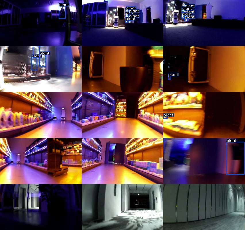
Obvious peaks. Auto-detect them, pull the frames at those moments, and run a detector (Moondream, one of the [VLM backends](/capabilities/perception)) to verify there really are plants:
```python skip session=robotdata theme={null}
from dimos.mapping.voxels import VoxelMapTransformer
from dimos.memory2.vis.space.space import Space
from dimos.memory2.transform import peaks
from dimos.memory2.vis.color import ColorRange
from dimos.memory2.vis.plot.elements import VLine
from dimos.memory2.vis.utils import mosaic
from dimos.memory2.stream import Stream
from itertools import chain
semantic_peaks = plantness_query_materialized.transform(peaks(key=lambda obs: obs.similarity, distance=1.0))
# load all lidar frames captured in the readius around the semantic peaks
# feed them into a global mapper to get a single pointcloud around our areas of interest
global_map = semantic_peaks \
.map(lambda obs: store.streams.lidar.near(obs.pose_stamped, radius=0.5).first()) \
.transform(VoxelMapTransformer()) \
.last().data
drawing = Space()
drawing.add(global_map)
drawing.add(semantic_peaks)
drawing.to_svg("assets/plot_plantness_autopeaks_map.svg")
peakColor = ColorRange("turbo")
for i, p in enumerate(semantic_peaks):
print(f"t={p.ts - plantness_similarity.first().ts:6.1f}s score={p.similarity:.3f} prominence={p.tags['peak_prominence']:.3f}")
plot.add(VLine(p.ts, color=peakColor(i)))
plot.to_svg("assets/plot_plantness_autopeaks.svg")
from dimos.models.vl.moondream import MoondreamVlModel
moondream = MoondreamVlModel()
moondream.start()
# peaks is still a stream of image observations (with prominence and semantic similarity metadata)
# so we can just draw it directly via mosaic that takes image streams
m = mosaic(semantic_peaks.map_data(lambda obs: moondream.query_detections(obs.data, "plant")))
m.data.save("assets/plants_auto.png")
```
```results theme={null}
14:59:33.042 [inf][dimos/mapping/voxels.py ] VoxelGrid using device: CUDA:0
t= 14.1s score=0.224 prominence=0.031
t= 26.3s score=0.225 prominence=0.033
t= 32.7s score=0.224 prominence=0.022
t= 37.0s score=0.259 prominence=0.067
t= 60.6s score=0.227 prominence=0.031
t= 61.5s score=0.218 prominence=0.026
t= 76.3s score=0.221 prominence=0.031
t= 84.0s score=0.223 prominence=0.027
t= 89.1s score=0.219 prominence=0.020
t= 162.9s score=0.224 prominence=0.041
t= 168.0s score=0.219 prominence=0.031
t= 172.4s score=0.218 prominence=0.020
t= 240.4s score=0.243 prominence=0.047
t= 245.6s score=0.224 prominence=0.028
t= 279.6s score=0.230 prominence=0.030
```
### Auto-detect the peaks and verify with a VLM
Obvious peaks. Auto-detect them, pull the frames at those moments, and run a detector (Moondream, one of the [VLM backends](/capabilities/perception)) to verify there really are plants:
```python skip session=robotdata theme={null}
from dimos.mapping.voxels import VoxelMapTransformer
from dimos.memory2.vis.space.space import Space
from dimos.memory2.transform import peaks
from dimos.memory2.vis.color import ColorRange
from dimos.memory2.vis.plot.elements import VLine
from dimos.memory2.vis.utils import mosaic
from dimos.memory2.stream import Stream
from itertools import chain
semantic_peaks = plantness_query_materialized.transform(peaks(key=lambda obs: obs.similarity, distance=1.0))
# load all lidar frames captured in the readius around the semantic peaks
# feed them into a global mapper to get a single pointcloud around our areas of interest
global_map = semantic_peaks \
.map(lambda obs: store.streams.lidar.near(obs.pose_stamped, radius=0.5).first()) \
.transform(VoxelMapTransformer()) \
.last().data
drawing = Space()
drawing.add(global_map)
drawing.add(semantic_peaks)
drawing.to_svg("assets/plot_plantness_autopeaks_map.svg")
peakColor = ColorRange("turbo")
for i, p in enumerate(semantic_peaks):
print(f"t={p.ts - plantness_similarity.first().ts:6.1f}s score={p.similarity:.3f} prominence={p.tags['peak_prominence']:.3f}")
plot.add(VLine(p.ts, color=peakColor(i)))
plot.to_svg("assets/plot_plantness_autopeaks.svg")
from dimos.models.vl.moondream import MoondreamVlModel
moondream = MoondreamVlModel()
moondream.start()
# peaks is still a stream of image observations (with prominence and semantic similarity metadata)
# so we can just draw it directly via mosaic that takes image streams
m = mosaic(semantic_peaks.map_data(lambda obs: moondream.query_detections(obs.data, "plant")))
m.data.save("assets/plants_auto.png")
```
```results theme={null}
14:59:33.042 [inf][dimos/mapping/voxels.py ] VoxelGrid using device: CUDA:0
t= 14.1s score=0.224 prominence=0.031
t= 26.3s score=0.225 prominence=0.033
t= 32.7s score=0.224 prominence=0.022
t= 37.0s score=0.259 prominence=0.067
t= 60.6s score=0.227 prominence=0.031
t= 61.5s score=0.218 prominence=0.026
t= 76.3s score=0.221 prominence=0.031
t= 84.0s score=0.223 prominence=0.027
t= 89.1s score=0.219 prominence=0.020
t= 162.9s score=0.224 prominence=0.041
t= 168.0s score=0.219 prominence=0.031
t= 172.4s score=0.218 prominence=0.020
t= 240.4s score=0.243 prominence=0.047
t= 245.6s score=0.224 prominence=0.028
t= 279.6s score=0.230 prominence=0.030
```

 ### Which peaks are significant?
We got 15 peaks back. Most prominences sit around 0.02-0.03 and only a couple (0.067 at t=37s, 0.047 at t=240s) really stand out. `significant()` replaces eyeballing that cutoff by thresholding on the distribution of prominences itself (default: MAD, median absolute deviation).
Once the surviving peaks go on the timeline, we get two very obvious plants:
```python skip session=robotdata theme={null}
from dimos.memory2.transform import significant
plot = Plot()
plot.add(
plantness_similarity.transform(smooth_time(5.0)).transform(normalize()),
label="plant-ness", color=color.green, gap_fill=0.0, connect=7.5,
)
meaningful_peaks = semantic_peaks.transform(significant(method="mad"))
for peak in meaningful_peaks:
plot.add(VLine(peak.ts, color=color.red))
m = mosaic(meaningful_peaks)
m.data.save("assets/plants_meaningful.png")
plot.to_svg("assets/plot_plantness_significant.svg")
```
### Which peaks are significant?
We got 15 peaks back. Most prominences sit around 0.02-0.03 and only a couple (0.067 at t=37s, 0.047 at t=240s) really stand out. `significant()` replaces eyeballing that cutoff by thresholding on the distribution of prominences itself (default: MAD, median absolute deviation).
Once the surviving peaks go on the timeline, we get two very obvious plants:
```python skip session=robotdata theme={null}
from dimos.memory2.transform import significant
plot = Plot()
plot.add(
plantness_similarity.transform(smooth_time(5.0)).transform(normalize()),
label="plant-ness", color=color.green, gap_fill=0.0, connect=7.5,
)
meaningful_peaks = semantic_peaks.transform(significant(method="mad"))
for peak in meaningful_peaks:
plot.add(VLine(peak.ts, color=color.red))
m = mosaic(meaningful_peaks)
m.data.save("assets/plants_meaningful.png")
plot.to_svg("assets/plot_plantness_significant.svg")
```

 Rule of thumb: keep a small absolute floor on `peaks(prominence=...)` to reject shape-noise, then let `significant()` pick the statistical cutoff.
### Zoom into a hotspot
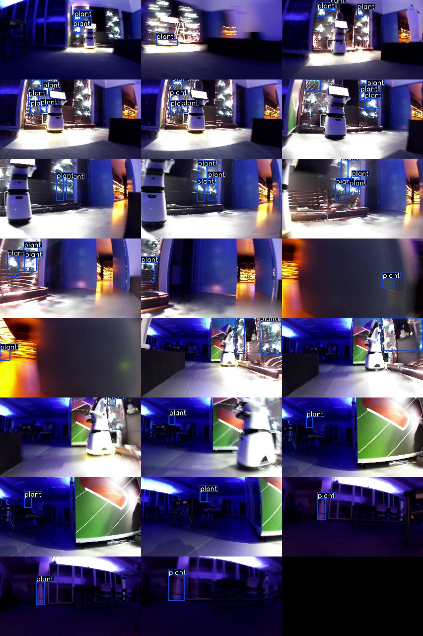
Focus on the strongest peak: load every image captured within 2.5 m of it (filtered for brightness and sharpness), rebuild the local 3D map from the lidar around it, and run the detector on all nearby views:
```python skip session=robotdata theme={null}
from dimos.memory2.vis.space.elements import Point
from dimos.memory2.transform import QualityWindow
drawing = Space()
# TODO actual near/at filters need to accept observation streams in order to easily
# reconstruct all frames in vicinity of another stream
# for now for simplicity here we are focusing only on one semantic hotspot.
meaningful_peak = meaningful_peaks.first()
# load all images captured in the readius around the semantic peak
near_images = images.near(meaningful_peak.pose_stamped, radius=2.5) \
.filter(lambda obs: obs.data.brightness > 0.1) \
.transform(QualityWindow(lambda img: img.sharpness, window=0.5))
# load all lidar frames captured in the readius around the semantic peak
# feed them into a global mapper to get a single pointcloud around our area of interest
global_map = store.streams.lidar.near(meaningful_peak.pose_stamped, radius=2.5) \
.transform(VoxelMapTransformer()) \
.last().data
# run our global mapper only on lidar frames around the POI
drawing.add(global_map)
drawing.add(meaningful_peak.pose_stamped, color=color.green)
# run a detector, filter small weird detections
detections = (near_images
.map_data(lambda obs: moondream.query_detections(obs.data, "plant"))
.map_data(lambda obs: obs.data.filter(lambda det: det.bbox_2d_volume() > 3000))
.filter(lambda obs: len(obs.data) > 0)
.materialize())
# materialize this stream since we'll want to re-use it later
drawing.add(detections)
drawing.to_svg("assets/peak_space.svg")
m = mosaic(detections)
m.data.save("assets/plants_peak_detections.png")
```
Rule of thumb: keep a small absolute floor on `peaks(prominence=...)` to reject shape-noise, then let `significant()` pick the statistical cutoff.
### Zoom into a hotspot
Focus on the strongest peak: load every image captured within 2.5 m of it (filtered for brightness and sharpness), rebuild the local 3D map from the lidar around it, and run the detector on all nearby views:
```python skip session=robotdata theme={null}
from dimos.memory2.vis.space.elements import Point
from dimos.memory2.transform import QualityWindow
drawing = Space()
# TODO actual near/at filters need to accept observation streams in order to easily
# reconstruct all frames in vicinity of another stream
# for now for simplicity here we are focusing only on one semantic hotspot.
meaningful_peak = meaningful_peaks.first()
# load all images captured in the readius around the semantic peak
near_images = images.near(meaningful_peak.pose_stamped, radius=2.5) \
.filter(lambda obs: obs.data.brightness > 0.1) \
.transform(QualityWindow(lambda img: img.sharpness, window=0.5))
# load all lidar frames captured in the readius around the semantic peak
# feed them into a global mapper to get a single pointcloud around our area of interest
global_map = store.streams.lidar.near(meaningful_peak.pose_stamped, radius=2.5) \
.transform(VoxelMapTransformer()) \
.last().data
# run our global mapper only on lidar frames around the POI
drawing.add(global_map)
drawing.add(meaningful_peak.pose_stamped, color=color.green)
# run a detector, filter small weird detections
detections = (near_images
.map_data(lambda obs: moondream.query_detections(obs.data, "plant"))
.map_data(lambda obs: obs.data.filter(lambda det: det.bbox_2d_volume() > 3000))
.filter(lambda obs: len(obs.data) > 0)
.materialize())
# materialize this stream since we'll want to re-use it later
drawing.add(detections)
drawing.to_svg("assets/peak_space.svg")
m = mosaic(detections)
m.data.save("assets/plants_peak_detections.png")
```

 ### Project detections into 3D
Finally, lift the 2D detections into 3D boxes on the map using the camera model and the pointcloud - from "the robot saw a plant at t=37s" to "there is a plant *here*":
```python skip session=robotdata output=none theme={null}
from dimos.perception.detection.type.detection3d.imageDetections3DPC import (
ImageDetections3DPC,
)
from dimos.robot.unitree.go2.connection import (
_camera_info_static as go2_camerainfo,
BASE_TO_OPTICAL,
)
from dimos.memory2.vis.space.elements import Box3D
from dimos.msgs.geometry_msgs.Pose import Pose
from dimos.msgs.geometry_msgs.Transform import Transform
from dimos.msgs.geometry_msgs.Vector3 import Vector3
# TODO We need a nicer way to get optical transform for image streams
# depending on the source
def world_to_optical(base_pose):
return -(Transform.from_pose("base_link", base_pose) + BASE_TO_OPTICAL)
drawing = Space()
drawing.add(global_map)
drawing.add(detections)
camera_info = go2_camerainfo()
detections3d = (detections
.map_data(lambda obs: ImageDetections3DPC.from_2d(
obs.data,
global_map,
camera_info,
world_to_optical(obs.pose_stamped),
))
.filter(lambda obs: len(obs.data) > 0))
# TODO detection3d needs to be a natural thing to render
for obs in detections3d:
for d3d in obs.data:
aabb = d3d.get_bounding_box()
c, e = aabb.get_center(), aabb.get_extent()
drawing.add(Box3D(
center=Pose(float(c[0]), float(c[1]), float(c[2])),
size=Vector3(float(e[0]), float(e[1]), float(e[2])),
color=color.green, label="plant",
))
drawing.to_svg("assets/peak_detections.svg")
```
### Project detections into 3D
Finally, lift the 2D detections into 3D boxes on the map using the camera model and the pointcloud - from "the robot saw a plant at t=37s" to "there is a plant *here*":
```python skip session=robotdata output=none theme={null}
from dimos.perception.detection.type.detection3d.imageDetections3DPC import (
ImageDetections3DPC,
)
from dimos.robot.unitree.go2.connection import (
_camera_info_static as go2_camerainfo,
BASE_TO_OPTICAL,
)
from dimos.memory2.vis.space.elements import Box3D
from dimos.msgs.geometry_msgs.Pose import Pose
from dimos.msgs.geometry_msgs.Transform import Transform
from dimos.msgs.geometry_msgs.Vector3 import Vector3
# TODO We need a nicer way to get optical transform for image streams
# depending on the source
def world_to_optical(base_pose):
return -(Transform.from_pose("base_link", base_pose) + BASE_TO_OPTICAL)
drawing = Space()
drawing.add(global_map)
drawing.add(detections)
camera_info = go2_camerainfo()
detections3d = (detections
.map_data(lambda obs: ImageDetections3DPC.from_2d(
obs.data,
global_map,
camera_info,
world_to_optical(obs.pose_stamped),
))
.filter(lambda obs: len(obs.data) > 0))
# TODO detection3d needs to be a natural thing to render
for obs in detections3d:
for d3d in obs.data:
aabb = d3d.get_bounding_box()
c, e = aabb.get_center(), aabb.get_extent()
drawing.add(Box3D(
center=Pose(float(c[0]), float(c[1]), float(c[2])),
size=Vector3(float(e[0]), float(e[1]), float(e[2])),
color=color.green, label="plant",
))
drawing.to_svg("assets/peak_detections.svg")
```
 That is the full loop: text query, temporal peaks, spatial hotspot, verified detections, 3D locations - all from one recorded drive, none of it requiring the robot again.
## Appendix: plotting API notes
Small things worth knowing about `Plot` when you build your own analyses.
Colors auto-cycle as you add series:
```python session=plot output=none theme={null}
import math
import random
from dimos.memory2.vis.plot.elements import Series
from dimos.memory2.vis.plot.plot import Plot
rng = random.Random(42)
xs = [i * 0.1 for i in range(120)]
color_check = Plot()
for i in range(14):
phase = rng.uniform(0, 2 * math.pi)
freq = rng.uniform(0.5, 1.8)
amp = rng.uniform(0.6, 1.4)
offset = i * 0.5 # vertical separation so curves don't overlap
ys = [amp * math.sin(freq * x + phase) + offset for x in xs]
color_check.add(Series(ts=xs, values=ys, label=f"curve {i + 1}"))
color_check.to_svg("assets/plot_colors.svg")
```
That is the full loop: text query, temporal peaks, spatial hotspot, verified detections, 3D locations - all from one recorded drive, none of it requiring the robot again.
## Appendix: plotting API notes
Small things worth knowing about `Plot` when you build your own analyses.
Colors auto-cycle as you add series:
```python session=plot output=none theme={null}
import math
import random
from dimos.memory2.vis.plot.elements import Series
from dimos.memory2.vis.plot.plot import Plot
rng = random.Random(42)
xs = [i * 0.1 for i in range(120)]
color_check = Plot()
for i in range(14):
phase = rng.uniform(0, 2 * math.pi)
freq = rng.uniform(0.5, 1.8)
amp = rng.uniform(0.6, 1.4)
offset = i * 0.5 # vertical separation so curves don't overlap
ys = [amp * math.sin(freq * x + phase) + offset for x in xs]
color_check.add(Series(ts=xs, values=ys, label=f"curve {i + 1}"))
color_check.to_svg("assets/plot_colors.svg")
```
 Named colors can also be used explicitly. When you pin a series to one of the named colors, the auto-cycle excludes it for the remaining series, so you never end up with two lines that share a color by accident:
```python session=plot output=none theme={null}
from dimos.memory2.vis import color
from dimos.memory2.vis.plot.elements import Series, HLine, Style
p = Plot()
# auto -> blue
p.add(Series(ts=xs, values=[math.sin(x) for x in xs]))
# explicit green, dotted
p.add(Series(ts=xs, values=[math.cos(x) for x in xs], color=color.red, style=Style.dotted))
# auto -> yellow (red is excluded)
p.add(Series(ts=xs, values=[math.sin(2 * x) for x in xs]))
# explicit color
p.add(HLine(y=0, style=Style.dashed, opacity=0.5, color="#ff0000"))
p.to_svg("assets/plot_named.svg")
```
Named colors can also be used explicitly. When you pin a series to one of the named colors, the auto-cycle excludes it for the remaining series, so you never end up with two lines that share a color by accident:
```python session=plot output=none theme={null}
from dimos.memory2.vis import color
from dimos.memory2.vis.plot.elements import Series, HLine, Style
p = Plot()
# auto -> blue
p.add(Series(ts=xs, values=[math.sin(x) for x in xs]))
# explicit green, dotted
p.add(Series(ts=xs, values=[math.cos(x) for x in xs], color=color.red, style=Style.dotted))
# auto -> yellow (red is excluded)
p.add(Series(ts=xs, values=[math.sin(2 * x) for x in xs]))
# explicit color
p.add(HLine(y=0, style=Style.dashed, opacity=0.5, color="#ff0000"))
p.to_svg("assets/plot_named.svg")
```
